Producing clean, reproducible sensorgrams is only half the challenge in kinetic binding experiments. Even the most carefully designed wet‑lab protocol can be undermined if the numerical methods used to analyse those traces, and the assumptions embedded in them, are not equally well understood. In practice, the numerical machinery that turns a raw response trace into a ka, kd and Rmax triple often deserves as much scrutiny as the experimental workflow that generated the data.
In the previous post in this series, we described how OpenBind developed a robust Creoptix GCI protocol that delivers well‑shaped, stable, and reproducible binding signals across a full production day. This post focuses on the other half: the affinity and kinetics data shipped with the data-release, how those data were generated, what exactly is included in the download, and critically where we still see open questions in the analysis. In particular, we want to surface an issue that is often implicit rather than explicit: how much do analysis choices: optimiser behaviour, initial parameterisation, and residual weighting – move the published numbers?
Where to find the data
Experimental Data Download:
- This Fragalysis-download-link will download about 600Mb of data, which contain the structures (aligned as described here) as well as affinities (look inside the extra_files_1 subdirectory). Further documentation for navigating the downloaded data can be found in Fragalysis-read-the-docs.
- Try this Fragalysis-data-view-link for a direct 3D view, which is fully documented here
- Detailed experimental protocols can be found on the OpenBind protocols.io Workspace
ML Data Download and Code:
Licencing and other useful links:
- Further information about OpenBind: https://openbind.uk/
- Data license: CC0 1.0 Universal
What’s in the Download, and How to Use It
The kinetics shipped in the first OpenBind data release are produced by the standard Creoptix workflow: the vendor software plus a trained human in the loop curating sensorgram fits cycle-by-cycle (i.e. the production pipeline). The values of the reported kinetics can be found in all_affinity_data_release_v1.csv`, which contains one row per analyte-cycle fit. Each row records:
- Run date: Date the experiment was performed
- Cycle number: Creoptix‑defined cycle identifier
- Protein concentration (μg/mL): Capture concentration of immobilised protein
- Channel: Signal channel in the format
Ch Y‑X, whereXis the reference channel andYthe active channel - Sample type: Control or test analyte
- ASAP IDs: ASAP identifier for the analyte
- OpenBind IDs: OpenBind analyte identifier
- SMILES: CxSMILES representation with enhanced stereochemical information
- Sample concentration (M): Analyte concentration used in the experiment
- ka (M⁻¹ s⁻¹): Association (on‑rate) constant estimated by Creoptix
- ka error (%): 95% confidence interval, expressed as a percentage of ka
- kd (s⁻¹): Dissociation (off‑rate) constant estimated by Creoptix
- kd error (%): 95% confidence interval, expressed as a percentage of kd
- KD (M): Equilibrium dissociation constant

- Rmax (pg/mm²): Maximum response estimated for the analyte
- Sqrt(Chi²): Square root of the Chi² goodness‑of‑fit metric
- Comments: Notes from the experimentalist regarding the fit or trace quality
- Used in analysis: Boolean flag indicating whether the data passed all curation criteria (defined in the notebook) or failed.
An SDF file `all_affinity_data_release_v1.sdf` was also generated from the CSV file, and contains the exact same information. The four original raw Creoptix experiment files can be found in the `creoptix_raw_data_release_v1.zip` archive.
The download also includes `sensofit_package_data_release_v1.zip`, a compressed file containing a more accessible format of the Creoptix raw data. It was generated by the `export_package` function of SensoFit (https://github.com/xchem/sensofit), an open-source Python tool developed by the OpenBind team that re-fits the same raw sensorgrams from scratch using a transparent, fully scripted numerical approach.
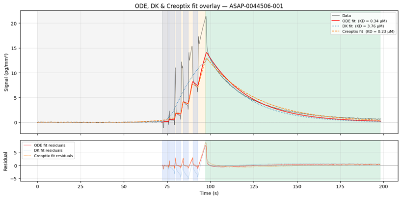
Along with the data files, a Jupyter Notebook, `sensofit_walkthough_data_release_v1.ipynb`, guides readers through reading, exploring, and using the data; and illustrates some of the current analysis challenges we are investigating; Figure 1 below was produced by this notebook and illustrates a raw sensorgram with different fitting approaches for a single representative compound as an example.
Finally, the `README` files in the download provide details about the contents of each file; and helps setting up the environment required to run the notebook and start the exploration of the data
Why Bother with a Second Fitter?
SensoFit does not claim to be a better analysis tool, it is a parallel, open view into how the fitting can be done; a sandbox for asking what the loss surface actually looks like, where the sensitivities are, and what it would take to reach into the regimes where the vendor software sometimes is unable to fit.
Pulsed waveform GCI sensorgrams are not what classical 1:1 Langmuir fitters were designed for. They contain three structurally different regions: a baseline before injection, an association phase made up of alternating analyte pulses (which carry buffer- & analyte-RI artefacts) and buffer pulses (which carry buffer-RI artefacts alone), and a dissociation phase after rinse-in, and the right way to fit each region is not the same.
The vendor software handles this elegantly for clean traces in the strong-to-moderate affinity regime, but two things are difficult to inspect from the outside: the choice of starting points fed into the underlying optimiser, and the impact of residual weighting applied across those three regions. Both of those choices, it turns out, can move the answer quite significantly in some cases.
SensoFit’s role, as illustrated by `sensofit_walkthough_data_release_v1.ipynb`, is to make those choices explicit and tweakable. It pairs a closed-form Direct Kinetics (DK) seeding step with a numerical Ordinary Differential Equation (ODE) multi-start fit of the 1:1 Langmuir model:
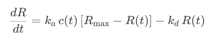
It uses a calibrated concentration function c(t) as well as a configurable residual mask to handle the analyte-pulse / buffer-pulse / dissociation split explicitly. It also reports per-phase goodness-of-fit metrics so that the trade-offs are visible rather than buried inside a single black-box number.
Room for improvements?
As captured in the notebook, the loss surfaces are not convex, and using DK-perturbed starts (the closed-form DK solution perturbed log-normally with in log-space) as opposed to fully random log-uniform starts offers tighter distributions because DK already sits in the right basin of attraction. The notebook also exposes the impact of the residuals weight assigned to the analyte pulses. While increasing the weights to “fit everything” generally gives a better fit on paper, the per-phases goodness-of-fit metrics show that improving the fit for the association phases leads to a decrease of the fit in the dissociation phases.
There is no objectively “right” answer falling out of the data alone, and that is precisely the open question we want to put in front of the community. SensoFit currently defaults to `association_weight = 0.0` (“dissociation-only” fitting) because it is the most robust to RI artefacts and the most directly comparable across compounds with different pulse-shape responses, but we hold that as a working choice rather than a verdict. Re-fitting the released data under a different weight is a one-line change in the notebook, and we would like to hear from anyone who has opinions on this.
What This Means for the EV‑A71 2A Data Release
The headline in this release come from the established Creoptix and human-curation pipeline; they are not an experimental output of SensoFit. What SensoFit and the accompanying notebook add is an open second look at the same raw traces; a way to ask, in code, how much the answer depends on the optimiser’s starting point, on the choice of residual weighting, and on the model assumptions baked into a 1:1 Langmuir fit.
Our view at OpenBind is that the right thing to do with those questions is not to settle them quietly behind closed doors and ship a single tidy column, but to ship the investigation alongside the data: the SensoFit code, the notebook, the per-cycle traces and the per-cycle fit diagnostics, so that anyone using this release for ML can re-fit, re-weight, or re-aggregate on their own terms and push back on our defaults.
A KD derived from a sensorgram is an interpretation; what matters for downstream modelling is whether the data is good enough to resolve the activity differences that matter, and whether the analysis is transparent enough to be argued with. The protocol post in this series handled the first half. SensoFit, and this blog post, are how we are opening the second half for the community to poke at.